A genetic connection matrix derived from kinship coefficients for the Indigenous populations of Mexico. Preliminary data from the MAIS cohort
The recruitment of individuals in the cohort was done with approval of the leaders of the Indigenous communities and with the help of the National Commission for the Development of Indigenous Communities of Mexico. All participants provided written consent and the authorities or community leaders were involved as translators. Findings from the study can be used by for-profit companies, according to the consent form. Sample collection for MAIS was approved by the Bioethics and Research Committees of the Insituto Nacional de Medicina Genómica in Mexico City (protocol numbers 31/2011/I and 12/2018/I). Preliminary data from the MAIS cohort have been discussed with the Indigenous leaders and volunteer individuals included in the study, explaining the meaning of the findings on health or population’s history, and the potential use of the data in future collaborations.
The maps of Mexico were created using the mxmaps R package. Variog from the GeoR R package was used to compute variograms on complex traits, with longitude and latitude used to compute distance (Supplementary Fig. 51).
ABCA1 variant frequencies were computed using plink in individuals from the MXB stratified by ancestry proxies from ADMIXTURE or by HDL cholesterol levels (Supplementary Fig. 59).
For each reference panel, we restricted the analysis to autosomes, removed all monomorphic SNPs, flipped all SNPs to the forward strand, and removed SNPs with an ambiguous strand.
The matrix was generated using kinship coefficients. As kinship estimates can be inflated under the presence of population structure and admixture, we obtained kinship coefficients for the genetic relationship matrix in the following manner: (1) PC-air75 was used to obtain principal components that capture ancestry and not relatedness (this procedure used kinship coefficients estimated using KING76 as input to partition samples into a related (5,562) and unrelated (271) set (using kinship threshold 0.044) and carrying out PCA on the unrelated set); (2) PC-relate77 was used to obtain kinship coefficients that capture relatedness but not ancestry (this method uses the ancestry-representative principal components from (1) to correct for population structure before calculating the kinship coefficients).
There are two random predictors in our model. The covariance structure and locality where the individual is from capture any other environmental variation not captured by the fixed predictors.
Extremes and negative values were removed from biochemical traits. Glucose was also checked against finger prick tests taken at the time of the survey, and values that were greatly discordant were also removed. Glucose measurements were further stratified by random or fasting glucose samples based on participant questionnaire responses.
Analyses of biometric data were used to make sure there were no outliers. The outliers were identified on the basis of their distribution density, and they ranged in height between 100 and 200 cm and weight from 25 to 300 kg.
Population-based genetic classifications for Mexican hypertension, arthritis and diabetes phenotypes based on a sample of 1000 Genomes genotypes
Binary health-related phenotypes were defined on the basis of questionnaire responses. Positive responses to the questionnaires were used as the basis for the definition of cases. Controls were those who responded with ‘no’. It was not possible for individuals to respond with do not know, pacifier not to answer or no response. Additionally, arthritis cases were defined as any individual with gout arthritis, rheumatoid arthritis and/or other forms of arthritis. Two hypertension phenotypes were defined: Hypertension_1, based on a diagnosis of hypertension; and Hypertension_2, which additionally took into account blood pressure readings. Cases were defined on the basis either a diagnosis for hypertension, medication or blood pressure readings greater than 140/90.
For each individual, we have access to data for various sociocultural factors such as access to healthcare and clean water, yearly income, educational attainment, whether they speak an Indigenous language or not, and whether they live in a rural or urban environment.
Localities were assigned values of latitude, longitude and altitude (metres) using data from the National Institute of Statistics and Geography (INEGI) in Mexico.
Although not intended, the groupings in use may seem to be similar to racial categories that were created in the past 500 years and used to justify European superiority and colonization of global regions. In Mexico, the history of racism and eugenics is similar to that in other parts of the world. We reject fixed hierarchical categorizations of humans, as well as their use to justify the superiority of one group over another. We use ancestry proxies that are estimated from ADMIXTURE using unsupervised clustering, as well as axes of ancestry that result from dimensionality reduction within these ancestries, capturing variation among groups from the Americas, for example. Genetics are continuous over time and space in humans, despite the confluence of genetic ancestries from around the globe in present-day Mexico.
The 1000 GenomesWGS genotype VCF files were downloaded from a server in the UK. 490 of those samples are in the MXL, CLM, PUR and PEL subpopulations. We constructed two subsets of genotypes on chromosome 2 from the Illumina HumanOmniExpressExome (8.v1-2) and Illumina GSA (v.2) arrays, and these were used as input to the TOPMed and MCPS10k imputation pipelines.
PCA with smartpca: Analysis of the 1000 Genomes Project Mexican ancestry sequences using Variant Effect Prediction and Admixture Bayes
The PCA was carried out by smartpca. Principal components generated by smartpca (Supplementary Figs. 6 and 7) were used to carry out the uniform manifold approximation and projection (UMAP) analysis (Fig. 1c and Supplementary Figs. 19 and 20)63. This analysis was done using a smartpca.
The 1000 Genomes Project Mexican ancestry cohort in Los Angeles, California repeated the analysis. The effect was to determine if it was due to ascertainment bias in the MEGAex array that covers fewer rare variants native to Mexico. The whole-genome sequences from the 1000 Genomes Project allowed us to rule this out. Ancestry estimates were generated using ADMIXTURE with reference panels from 1000 Genomes (CEU: Utah residents (CEPH) with Northern and Western European ancestry, GBR: British in England and Scotland, YRI: Yoruba in Ibadan, Nigeria and PEL: Peruvian in Lima, Peru) and 50 whole-genome sequences of Indigenous individuals across Mexico generated as part of the MXB Project65. Variant effect predictor was used to annotate SNPs, and mutation burden was computed in the same manner. The term stop gained or stop lost is one of the consequence terms in the deleterious category.
Using AdmixtureBayes, we inferred the split events and admixture events that have occurred in the MXB. We used the default parameters for generating the admixture graph with the exception of the number of chains and iterations, which we set to a higher value of 16 (–MCMC_chains 16) and 20,000 (–n 20000) to ensure convergence; we also used the -slower flag, enabling the computation of the necessary information to plot the top trees, and a burn-in period corresponding to half the samples. The tree was plotted with the highest possible probabilities, which allowed us to explore the uncertainty of the inferences. The AdmixtureBayes method can be found in the corresponding paper.
Variation effect predictors for the sum of ROH by geographic and birth year in the XXB. A study using FUMA SNP2GENE
ROH were also correlated with birth year in the MXB (Fig. 3d) The variable was used in the analysis. The first two decades were taken out of the analysis due to the number of individuals who did not sample in this period. Birth year was also directly correlated with ancestries from the Americas (inferred using ADMIXTURE) in rural and urban localities separately. The correlation of ROH with global ancestries per individual was shown in the supplementary figs. An R script was used to analyse distributions of the sum of ROH by geography (Supplementary Figs. 31 and 33).
The variant was described as previously described38. The most severe consequence for each variant chose across all transcript was used in the annotated variant effect predictor. In addition, we created annotations from a combination of MANE, APPRIS, and Ensembl tags. MANE annotation was given the highest priority followed by APPRIS. The definition of Ensembl was used when neither MANE nor APPRIS annotations were available. Gene regions were defined using Ensembl release 100. The allele of interest was not the ancestral one, which caused the loss-of-function variants to be annotated. PolyPhen2 HVAR, SIFT, and PolyPhen2 HDIV were assigned deleteriousness by using the five resources. Missense variants were considered ‘likely deleterious’ if predicted deleterious by all five algorithms, ‘possibly deleterious’ if predicted deleterious by at least one algorithm and ‘likely benign’ if not predicted deleterious by any algorithm.
Lead association SNPs and potential causal groups were defined using FINEMAP (v1.3.1; R2 = 0.7; Bayes factor ≥ 2) of SNPs within each of these regions on the basis of summary statistics for each of the associated traits70. FUMA SNP2GENE was then used to identify the nearest genes to each locus on the basis of the linkage disequilibrium calculated using the 1000 Genomes EUR populations, and explore previously reported associations in the GWAS catalogue40,71 (Supplementary Table 7).
Long-term storage and isolation of plasma and buffy-coat DNA for a prospective cohort study of the health effects of tobacco use in Mexico
The British and Mexican scientists at the University of Oxford had discussions in the late 1990s about what to do about the health effects of tobacco in Mexico. The plan was to establish a prospective cohort study that would investigate both the health effects of tobacco and other factors as well. Tens of thousands of women and men 35 years old or older agreed to take part in the study, which involved physical testing, blood samples, and questions about mortality. More women than men are in the study because the study visits were mostly done during working hours when women were more likely to be at home.
Blood samples were obtained from everyone at the recruitment stage and then taken to a central laboratory where they were transferred to a transport box with ice packs. Samples were refrigerated overnight at 4 °C and then centrifuged (2,100g at 4 °C for 15 min) and separated the next morning. Plasma and buffy-coat samples were stored locally at −80 °C, then transported on dry ice to Oxford (United Kingdom) for long-term storage over liquid nitrogen. The buffy coat’s genes were suspended in the TE buffer and were prepared using Perkin-Elmer Chemagic systems. UV-VIS spectroscopy using Trinean DropSense96 was used to determine yield and quality, and samples were normalized to provide 2 μg DNA at 20 ng μl–1 concentration (2% of samples provided a minimum 1.5 µg DNA at 10 ng µl–1 concentration) with a 260:280 nm ratio of >1.8 and a 260:230 nm ratio of 2.0–2.2.
Genomic samples were transferred to the Genetics Center from the UK Biocentre and they were stored in a biobank at – 80C for sample preparation. All DNA libraries were created using a common Y- shaped adapter and by enzymatically shearing the entire DNA to a small fragment. Unique, asymmetric 10 bp barcodes were added to the DNA fragment during library amplification to facilitate multiplexed exome capture and sequencing. All samples were captured on the same lot of oligonucleotides after equal amounts of sample were pooled. The captured DNA was PCR amplified and quantified by quantitative PCR. The multiplexed samples were pooled and then sequenced using 75 bp paired-end reads with two 10 bp index reads on an Illumina NovaSeq 6000 platform on S4 flow cells. More than 147,000 samples were made available for processing. We were unable to process more than two thousand samples due to low or noDNA being present. A total of 143,440 samples were analyzed. The average 20× coverage was 96.5%, and 98.7% of the samples were above 90%.
We separately phased the support-vector-machine-filtered WES and WGS datasets onto the array scaffold. The reference panel is made up of the phased WGS data. The information we got from the sequence reads and the subset of available trios were fed into Shapeit. Phasing was carried out in chunks of 10,000 and 100,000 variants (WES and WGS, respectively) and using 500 SNPs from the array data as a buffer at the beginning and end of each chunk. The use of the phased scaffold of array variants meant that chunks of phased sequencing data could be concatenated together to produce whole chromosome files that preserved the chromosome-wide phasing of array variants. The data from the array dataset was used when there was a variant in the array, and there was a variant in the Sequencing dataset.
We implement a supervised machine-learning function to discriminate between low-quality and high-quality variants. In brief, we defined a set of positive control and negative control variants based on the following criteria: (1) concordance in genotype calls between array and exome-sequencing data; (2) transmitted singletons; (3) an external set of likely ‘high quality’ sites; and (4) an external set of likely ‘low quality’ sites. To define the external high-quality set, we first generated the intersection of variants that passed QC in both TOPMed Freeze 8 and gnomAD v.3.1 genomes. The GATK resource bundle gave access to a previous study and high confidence SNPs from the 1000 Genomes project, which were restricted to this set. We used a combination of fail and duplicate variants to define the low-quality set. When model training began, the control set of variants were binned and randomly sampled so that an equal number of them were retained in the positive and negative labels. A support machine using a radial basis function was then trained on up to 33 site quality metrics, which included the median value for allele balance in heterogeneous calls and if a variant was split from a multi-allelic site. We split the data into training (80%) and test (20%) sets. We performed a grid search with cross-validation on a training set and used the hyperparameters from that set to confirm the accuracy of the test set. This approach identified a total of 616,027 WES and 22,784,296 WGS variants as low-quality (of which 161,707 and 104,452 were coding variants, respectively). We used a set of hard filters to exclude monomorphs, unresolved duplicate, variant with 1% missingness, and failed Hardy–Weinberg equilibrium.
We used Shapeit (v.4.1.3; https://odelaneau.github.io/shapeit4) to phase the array dataset of 138,511 samples and 539,315 autosomal variants that passed the array QC procedure. To improve the phasing quality, we leveraged the inferred family information by building a partial haplotype scaffold on unphased genotypes at 1,266 trios from 3,475 inferred nuclear families identified (randomly selecting one offspring per family when there was more than one). We then ran Shapeit one chromosome at a time, passing the scaffold information with the –scaffold option.
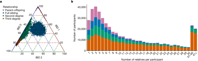
We used the phased array dataset of over 137,000 samples and over 538,614 sites to identify IBD segments. Hap-ibd was run with the parameter min-seed=4, which looks for IBD segments that are at least 4 cM long. The procedure in IBDkin shows us how much overlap there is in some regions and how much less overlap there is in others. The sample was plugged into the exome data for a loss-of-function variant evaluation, resulting in a 136,200 sample. We further overlaid the ROH segments with local ancestry estimates, and assigned ancestry where the ancestries were concordant between haplotypes and posterior probability was >0.9, assigning ancestry to 99.8% of the ROH.
To apply to the IBD network of the MCPS cohort, we first removed edges with weight >72 cM as previously done14. The visualization was created to avoid being influenced by extended families. We then computed the eigenvectors of the Laplacian graph after getting the biggest connected component from the IBD network.
We imputed the filtered array dataset using both the MCPS10k reference panel and the TOPMed imputation server. For TOPMed imputation, we used Plink2 to convert this dataset from Plink1.9 format genotypes to unphased VCF genotypes. For compatibility with TOPMed imputation server restrictions, we split the samples in this dataset into six randomly assigned subsets of about 23,471 samples, and into chromosome-specific bgzipped VCF files. Six jobs have been submitted to the TOP Med imputation server using the NIH Biocatalyst API. Following completion of all jobs, we used bcftools merge to join the resulting dosage VCFs spanning all samples. For the MCPS10k imputation, we used Impute5 (v.1.1.5). The window size and buffer size for the imp5Chunker program is 500 kb and 5 MB, respectively. There was a method for calculating information scores that was available on the well.ox.ac.uk.
mathop’sum limits_j=12p
Source: Genotyping, sequencing and analysis of 140,000 adults from Mexico City
Estimating exome singleton sites in the UK Biobank cohort with application to whole genome regression in MCPS individuals with type 2 diabetes
The sample size for population k at the site is estimated. Existing methods can be difficult to phase. The amount of singleton sites was increased with the help of family information and phase information in the WGS phase. In the WES dataset, we found that the majority of exome singletons occurred in areas where there are lots of descendants of the same race. For these variants, we gave equal weight to the two ancestries when estimating allele frequencies.
$$\begin{array}{l}{V}{l}\,=\,{{(i,j)}{l}:{\rm{for}}\,1\le j\le 2\,{\rm{and}}\,1\le i\le N}\ {E}{l}\,=\,{({(i,j)}{l},{(s,t)}{l}):{h}^{{(i,j)}{l}}\,{\rm{and}}\,{h}^{{(s,t)}_{l}}\,{\rm{are}}\,{\rm{IBD}}}.\end{array}$$
$$\begin{array}{l}W={\sum }{C\in {C}{{\rm{ALT}}}}{\bar{p}}{C}\ N={\sum }{C\in {C}{{\rm{ALT}}}}{\bar{p}}{C}+{\sum }{C\in {C}{{\rm{REF}}}}{\bar{p}}_{C}\end{array}$$
A predominantly European-ancestry cohort from the UK Biobank was used to conduct whole genome regression in individuals in the MCPS. Individuals with type 2 diabetes were not included. All the models were adjusted for age, age2, and technical covariates as well as the rank-based inverse normal transformation. The summary statistics from the UK Biobank were used to make aBMI PR in MCPS; on the other hand, theMCPS summary statistics were applied to UK Biobank statistics.