A comparison of references for deconvolution within normal and tumour brain Visium samples from the Spatial LIBD Project using the Human Stem Cell Dataset

The human stem cell dataset was analysed using the same parameters as in the tumorigenesis atlas dataset, only with human orthologues. The same quality control cutoffs as for our atlas were used; Seurat and Harmony were used to integrate, correct batch effects, and cluster cells together. The same computational Pipeline was used for calculating the top differentially expressed genes.

For the human Visium samples, which consist of late-stage tumours with almost no normal regions, we turned to the normal brain Visium data from the SpatialLIBD Project. To mitigate potential reference biases, we randomly selected two slides from the project as references, conducted inferCNV independently for each, and compared the results. Both references yielded congruent outcomes.

Scanpy v1.9.3 and squidpy v1.3.0 were used to analyse spot genes in Visium. We used a single-cell mouse datasets for our reference for deconvolution within each spot. For mouse Visium samples containing both normal and tumour regions, an initial reference was constructed using the major cell types denoted in Fig. 1c. The results of the analysis proved that the cancer was from normal regions. Two seperate references for the tumours and normal regions were created to get a more detailed deconvolution of the cells. For the reference, the cells of the tumor were removed and replaced with other cells. Subtypes labels were used to build the tumour reference. This reference was made using normal brain cell types.

When estimating the reference cell type signatures, the ‘sample ID’ served as the batch_key to mitigate batch effects. The total UMI count and theMitochondrial gene ratio were included to counteract potential biases. After these references were established, we performed the deconvolution separately for tumour and normal regions using their respective references. For human samples, as all tissues were sourced from tumour regions, the tumour reference was used for deconvolution.

We used the R package rstatix (v0.7.0) to compute the one-sided Fisher’s exact tests of the proportions of the cell types in the different time points. For each time point, we calculated the number of cells in each cell category to construct the contingency table. The function fisher_test was used to perform the tests.

The cells from the aged libraries have no annotations because they have already been published and annotated. We mapped all aged cells to the ABC-WMB reference taxonomy as previously described3. Briefly, we assigned their cell-type identities by mapping them to the nearest cluster centroid in the reference taxonomy using the corresponding Annoy index using the same method as implemented at present in the R package scrattch.mapping. We also used this approach for assigning cell-type identities for cells segmented from Resolve spatial data to the ABC-WMB cell-type taxonomy or external datasets as reference, using different gene lists based on the contexts. We used a list of prominent marker genes from the reference cluster to assemble a list of 72 genes that were added to the microglia dataset. When a mapping confidence score was needed, we did a random sample of 80% genes from the marker list. We define the fraction of times a cell is assigned to a given cell type as the mapping probability to that type.

All libraries were 10xv3 samples and processed as previously described3,20. All libraries were mapped to the mouse reference using the 10x Genomics CellRanger pipeline with the include introns argument. This resulted in an scRNA-seq dataset containing 2,777,165 cells.

Nested clustering with three different distance measures of the shortest path distance on a tree was used as one of the methods to reconstruct the cell phylogeny. MED was calculated using a formula called MEDALT. The tree was loaded into R as an Igraph object and visualized with GGally and igraph.

The CNAs in a cell are acquired in two ways: inherited from its parent cell; newly acquired during cell division. We did a simulation on the whole tree. For each of the cells, we assume a random distribution with the number of newly acquired CNAs followed by a. This means that with probability e−λ, a cell will not get any new CNA. In our simulation, λ was set between 0.1 and 0.5. CNAs can affect contiguous sites and regions in a chromosome, meaning that a gain (or loss) of copy for adjacent genes can happen together. In our simulation, a mean of 100–200 genes were predicted to follow the number of genes that one CNA affected. After each simulation, CNAs for living cells were selected for downstream analysis.

The classic birth death process and immigration process were recreated using two models. The second model has been proved to explain cell growth dynamics in the tumour context when there is a proliferative hierarchy with a stem cell-like population.

in which N0 is the initial number of cells, and b and d are the birth and death rate, respectively. The interval of time between the events is followed by an exponential distribution. When branching happens, it can be a birth with a probability of b/(b + d), or a death with a probability d/(b + d). In our simulation, we assumed that the birth and death rates do not change during the evolution.

Differential analysis of the cell-cell communication in tumorigenesis using CellChat and phateR packages v1.1.338

We used CellChat v1.1.338 for the analysis of cell–cell communication, which was performed separately for each of the four stages of tumorigenesis. We followed the official workflow with default parameters unless otherwise indicated. The first thing we did was load the normalized counts into CellChat, followed by the preprocessing steps. We smoothed gene expression by applying a diffusion process on the protein–protein interaction network implemented in projectData() function. The computeCommunProb function was run to eliminate possible bias due to cell population size. This resulted in a network of communication strength between all cell states for each of the ligand–receptor pairs that passed the filtering steps. To determine the communication strength between cell states, we used aggregation functions. For each of the pathways (data slot netP), we evaluated the role of different cell states as senders or receivers on the basis of the out-degree or in-degree of the communication network, implemented in the netAnalysis_signallingRole() function.

The R packages phateR v1.0.765 and slingshot v1.8.066 were used to build trajectories. First, we used phateR to generate two-dimensional (2D) embeddings (PHATE space), with the 50 harmony embeddings as input. We built a tree of cell types using slingshot. For differential analysis, we first clustered cells into five clusters along the trajectory, and then the cluster-specific maker genes were found using the FinderAllMarkers() function in Seurat. The K-nearest neighbours were used to test the results, and they were summarized via PAGA. All of these methods resulted in similar topologies between cell states.

Source: Gliomagenesis mimics an injury response orchestrated by neural crest-like cells

Study of Transgenic Mice in a 12-h Dark-light Cycle Facility at Jackson Laboratories. I. MRI characterization of glioma and control mice

The transgenic mice used in this study were obtained from Jackson Laboratories, with the following exceptions: Sox2creER (B6;129S-Sox2tm1(cre/ERT2)Hoch/J) from Konrad Hochedlinger56; Trp53f/f from Chi-chung Hui57; Sox2eGFP (Sox2tm1Lpev) from Freda Miller58. The glioma and control mouse model were housed in 12-h dark–light cycle facilities that provided free access to water and chow and maintained the appropriate temperature and humidity. The mice were monitored and euthanized when they developed symptoms of intracranial pressure or focal neurological abnormality. The ethical and legal regulations were followed in the mouse experiments. The experiments and animal use protocols were approved by the Animal Care Committees in the different institutions at the University of Toronto, including the Hospital for Sick Children and University Health Network.

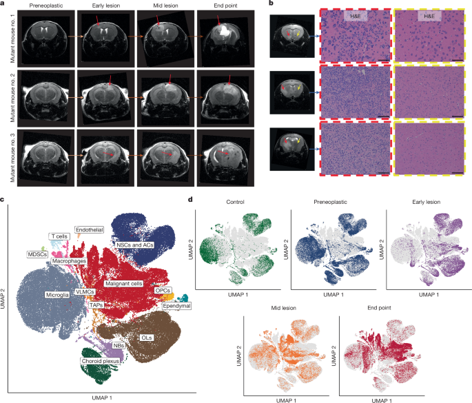
MRI was performed as reported previously8, and fresh brain tissue was collected from mutant mice at four MRI-defined stages: the ‘preneoplastic’ stage, at which the brain imaging shows no signs of neoplastic lesion development; the ‘early-lesion’ stage, characterized by small abnormalities seen on T2-FLAIR MRI sequences; the ‘mid-lesion’ stage, when the lesion has reached a larger size, as indicated by a T2-FLAIR-bright mass, in asymptomatic animals and occupies a substantial fraction of the brain hemisphere; and, finally, the ‘end-point’ stage, when mice develop symptoms of raised intracranial pressure or focal neurological abnormalities, with the tumour extending over a large portion of the brain hemisphere(s), typically with midline shift. The sample of brain tissue was divided into single cells. This was followed by FACS to separate the live tdTomato+ cells and tdTomato− cells. Following sorting, both populations were characterized by scRNA-seq using the 10x Genomics platform as reported previously8. Tissue processing and cell sorting were done the same way as for the mouse brain injury samples. The cells with GFP. For scATAC-seq, the nuclei were isolated from sorted cells and then processed using the 10x Genomics Single Cell ATAC-seq Workflow and following the manufacturer’s protocol. The added 5 l of nucleic suspension was used for the gel beads-in-emulsion (GEMs) generation and barcoding on the 10x Chromium Chip E. The DNA was recovered using Dynabeads MyOne Silane beads. Libraries were validated on the Agilent 2100 Bioanalyzer to check for size and quantified by quantitative PCR using Kapa Library Quantification Illumina/ABI Prism Kit protocol (KAPA Biosystems). Illumina recommended that libraries be pooled in equimolar quantities and used to generate pairs of reads of 50 bases in length. Spatial transcriptomics was performed on formalin-fixed and paraffin-embedded mouse tissue sections using the 10x Genomics Visium platform and following the manufacturer’s protocols (user guides CG000407 Rev D and CG000409 Rev C).

The mice were ready to be operated on. The intracranial osmotic pump was implanted following the instructions of the manufacturer, though it had been implanted at 1.5 MM to 3.0 MM. The osmotic pump is filled with normal saline and the brain will be infused at a flow rate of half a liter h1 for a week.

Differential Analysis of Precursor-like Malignant States with Integrated FastMNN60, BBKNN61 and EdgeR24

To make sure downstream analysis is not biased by the integration method, we used FastMNN60, which is implemented in a SeuratWrappers, andBBKNN 61, which is implemented in a Scanpy62. All of the methods gave the same results.

To explore the heterogeneity within the cycling PC-like cells, we first isolated these cells from the malignant cells and then removed all cell cycle mouse orthologues associated with both S and G2/M phases63 as well as all of the genes from the KEGG (Kyoto Encyclopedia of Genes and Genomes) cell cycle pathway reference (https://www.genome.jp/entry/pathway+mmu04110). The 205 cell cycle genes had to be removed because they were expressed at high levels. Six cycling cell types were revealed by clustering: NSC-, cycling OPC-, cyclingNPC-, cycling MSC-, and cycling AC-. To compute the fractions of cycling and non-cycling cells for each of the precursor-like malignant states (NSC, OPC, NPC, MSC and NCC), we calculated the number of cycling and non-cycling cells for each precursor state in each of the samples. The PC-like fractions of both cycling and non-cycling cells were calculated as a number of cells over the sum of both cycling and non-cycling cells. The averages were plotted along with their standard errors.

Each of the tumours had relative CNA stored in Seurat as a “modality” and processed with the log-normalization pipeline. We therefore obtained a new set of PCA embeddings, clusters and UMAP visualizations. There are different cell states in most of the CNA clusters. We fed the PCA embedded into the miloR package to further elaborate on this. The neighbourhood index cell colour and size are calculated by the number of cells in the neighbourhood, while the neighbourhood colour is based on the state of the cell. The number of cells is shown in the graph edges.

We also performed differentially expressed gene analysis at the pseudo-bulk level with R package EdgeR24 (v.3.32.1). Mean gene expression was calculated for each cell type and library combination. We fit a simple model using EdgeR’s likelihood ratio test and default parameters. The examples that are shown in the table are calculated from EdgeR. 6a,b and correlations with age effect sizes estimated from MAST are summarized in Extended Data Fig. 6c.

where age and sex are all categorical variable each with two levels, and gene detection (gc) and QC score (qc) are log transformed and then z-score normalized, and the tilde (~) means distributed as. We included both gene detection and QC score in each model to account for potential effects that various FACS population plans had on library quality (Extended Data Fig. 6e,f). The P values were generated from the likelihood ratio test between the different models. The Bonferroni correction corrected the P values. The log2FC of each gene can be seen in the main body of the text asage effect size, which is defined as the age term for each model.

Computing and analysing brain regions using in situ spatial RNA data from the Resolve Biosciences Molecular Cartography (MMAP) platform

We used the principal components calculated from PCA to calculate UMAPs. We performed PCA on UMAPs with over 100,000 cells by using a matrix of genes and top markers from each cluster. There was no imputation for UMAPs with less than 100,000 cells. The number of principal components, the size of the local neighbourhood of cells and the structure of the data are all parameters that can be adjusted when generating UMAPs. For all UMAPs, the top 150 principal components were chosen and principal components with more than 0.7 correlation with technical bias were removed. Each PCA was run with a unique gene list and each UMAP was run with a different set of nn.neighbours and md parameters. The parameters used for each PCA/UMAP were as follows: 6,446 genes, nn.neighbours = 20, md = 0.5 for the global UMAP (Fig. 1); 984 genes, nn.neighbours = 20, md = 0.5 for the OPC-Oligo UMAP (Fig. 3); 1,884 genes, nn.neighbours = 5, md = 0.5 for the Immune UMAP (Extended Data Fig. 10); 1,806 genes, nn.neighbours = 20, md = 0.5 for the Astro-Epen UMAP (Fig. 4); 401 genes, nn.neighbours = 5, md = 0.5 for the tanycyte and ependymal cell UMAP (Fig. 4); 1,169 genes, nn.neighbours = 5 and md = 0.5 for the HY (hypothalamus) neuron UMAP (Fig. 5).

By using the numbers of adult and aged cells per cluster we could determine if the clusters were made up of more cells than expected.

All in situ spatial RNA data shown here were generated by Resolve Biosciences with their commercially available Molecular Cartography platform. There were four experiments which used a different panel of 100 genes and targeted different regions of the brain. For RSTE1, four different regions of the brain (cortex, striatum, midbrain and hindbrain) were imaged in both sexes and both ages (2 and 18 months), with two replicate brains per condition and two technical replicates per brain. Independent replicates were plotted and analysed in all figures. For RSTE2, the RSP and hippocampus were imaged in both sexes and ages, with four replicate brains per condition. For RSTE3 and RSTE4, the hypothalamus was imaged in both sexes and both ages, with four replicate brains per condition. Brain dissection and cryosectioning for Molecular Cartography experiments were performed at the Allen Institute for Brain Science in Seattle, WA, samples were stored at −80 °C for 1–3 days, and then shipped overnight to Resolve Biosciences in San Jose, CA, USA where the Molecular Cartography protocol was performed. Spot data were then made available 1–2 weeks after receipt of tissue. There were methods used for data analysis at the Allen Institute. In order to split transcript data into different types of cells, various quality metrics were generated, and visualization and analysis was done.

The brains of the fresh-frozen adult and aged were sectioned at 10 m. The OCT block containing a fresh-frozen brain was trimmed in the cryostat until reaching the desired region of interest. Sections were placed onto coverslips provided by Resolve Biosciences. Two replicate sections were collected sequentially: one as the primary sample and the other as a backup.

Cells were divided using a combination of open-source software. Cellpose uses a generalist algorithm for segmenting cells from images of cellular stains as input. To draw cell boundaries Baysor uses transcript data alone and also has an option of integrating previous knowledge from stained images into the process. The images from the tissue samples were used to train the model for Cellpose. The output of Cellpose was used as a starting point for Baysor. Baysor was run with the following input parameters: -m 30, -s 50.

We used a strict quality control process to remove the low-quality cells. Cells were first filtered by a broad set of quality cut-offs based on gene detection, QC score and doublet score. A set of genes are summed up by log-transformed expression and their expression level is compared against cells that have a better expression level. Briefly, these are housekeeping genes that are strongly expressed in nearly all cells with a very tight coexpression pattern that is anticorrelated with the nucleus-enriched transcript Malat1. We can quantify the integrity of the mRNA content with this score. Doublets were identified using a modified version of the DoubletFinder algorithm89. For this preliminary round of filtering, we included cells with gene detection greater than 1,000, a QC score greater than 50 and a doublet score less than 0.3. Using these thresholds, 1,999,976 cells remained in the dataset (Extended Data Fig. 3a). The visualization shows the mix of cell types by library and other categories.

For 10xv3 processing, we used the Chromium Single Cell 3′ Reagent Kit v.3 (1000075, 10x Genomics). We followed the manufacturer’s instructions for the construction of a library. We targeted a sequencing depth of 120,000 reads per cell; the actual average achieved was 77,743 ± 36,025 (mean ± s.d.) reads per cell across 287 libraries (Supplementary Table 1).

To enrich for neurons or live cells, cells were collected by FACS (BD FACSAria II or FACSAria Fusion, with FACSDiva v.8 software) using a 130 μm nozzle. Cells were prepared for sorting by passing the suspension through a 70 µm filter and adding Hoechst or 4,6-diamidino-2-phenylindole (DAPI) (to a final concentration of 2 ng ml−1). The sorting strategy was as previously described3,20, with most cells collected using the tdTomato-positive label. A tube containing 500 liters of quenching buffer was used to sort the 30,000 cells. We found that cell death was caused by the ACSF being in the collection buffer. We also observed decreased cell viability for longer sorts. Each aliquot of sorted 30,000 cells was gently layered on top of 200 µl of high BSA buffer and immediately centrifuged at 230g for 10 min in a centrifuge with a swinging bucket rotor (the high BSA buffer at the bottom of the tube slows down the cells as they reach the bottom, minimizing cell death). The supernatant and 35 l of buffer were left behind after we resuspended the cells. Immediate centrifugation and resuspension allowed the cells to be temporarily stored in a high BSA buffer with minimal ACSF dilution. The resuspended cells were stored at 4 °C until all samples were collected, usually within 30 min. There was pooled samples, cell concentration quantified and immediately loaded onto the 10x Genomics Chromium controller.

Tissue pieces were broken down into small pieces to be eaten with 30 U liter of papain. For 30 minutes, PAP2 is in ACSF. Due to the short time in a dry oven, we set the temperature to 35 C to compensate for the indirect heat exchange, and set the solution temperature to 30 C. Enzymatic digestion was quenched by exchanging the papain solution three times with quenching buffer (ACSF with 1% fetal bovine serum and 0.2% bovine serum albumin (BSA)). Samples were incubated on ice for 5 min before trituration. The tissue pieces in the quenching buffer were triturated through a fire-polished pipette with a 600 µm diameter opening roughly 20 times. The tissue pieces were allowed to settle and the supernatant, which now contained suspended single cells, was transferred to a new tube. Trituration and supernatant transfer could be done using 300 and 150 m fire-polished pipettes. The single-cell suspension was passed through a 70 m filter into a 15ml conical tube, with a high BSA buffer at the bottom of it to help cushion cells during centrifugation at 100g. The cell pellet was resuspended in the quenching buffer after the supernatant was discarded. We collected 1,508,284 cells without performing FACS. The cells were immediately loaded onto the 10X Genomics controller after they had been quantified.

The procedure for isolating single cells was adapted previously. The brain was dissected, submerged in artificial cerebrospinal fluid (ACSF), embedded in 2% agarose and sliced into 350-μm coronal sections on a compresstome (Precisionary Instruments). Block-face images were captured during slicing. ROI were then microdissected from the slices and dissociated into single cells. Before and after the dissection, images of each slice were taken. These images were used to document the precise location of the ROI using annotated coronal plates of CCFv3 as reference.

All procedures were carried out in accordance with Institutional Animal Care and Use Committee protocols at the Allen Institute for Brain Science. Mice were provided food and water ad libitum and were maintained on a regular 14/10 h day/night cycle at no more than five adult animals of the same sex per cage. Ambient temperature of the vivarium was maintained between 21.1 and 22.78 °C (70–73 °F) and humidity was maintained between 40 and 45%. There were mice on the C57BL/6J background. We excluded any mice with dermatitis, anophthalmia, microphthalmia, seizures or abdominal masses.

We used 44 aged mice (20 female, 24 male) and 64 young adult mice (31 female, 33 male) to collect cells for 10xv3 scRNA-seq. All young adult mice were also included in the ABC-WMB atlas3. Aged animals were euthanized at P540–553 (roughly 18 months) and young adult animals were euthanized at P53–69 (roughly 2 months). No statistical methods were used to predetermine sample size. All donor animals used in this study are listed in Supplementary Table 1. The Zeitgeber time of the light/dark cycle was similar (within a 3 h window) for all the tissue collections. We didn’t keep a record of the cycle for female mice.

We isolated nearly 300 libraries from more than 100 animals. All libraries are listed in Supplementary Table 1. The Transgenic driver lines were used to enrich cell isolation. Roughly half the libraries (n = 145) were sorted for neurons from the pan-neuronal Snap25-IRES2-Cre line (JAX strain no. 023525) crossed to the Ai14-tdTomato reporter. Supplementary Table 1. We did not use enriched libraries for unbiased sampling, but we used a variety of different types of mice, including wild type C57BL/6J mice. Unbiased sampling techniques include libraries that were stained and sorted for Hoechst+, Calcein+ or unstained libraries that were not sorted at all. No FACS cells make up roughly 25% of the final high-quality dataset. The transgenic Snap25-IRES2-Cre line was backcrossed to C57BL/6J for at least ten generations before crossing and can be considered congenic. The Ai14 line was cross-crossed at least five generations before being considered incipient congenic. gating strategies can be seen in the examples in Extended Data.

We used the CCFv3 (RRID: SCR_002978) ontology22 (http://atlas.brain-map.org/) to define brain regions for profiling and boundaries for dissection. We carefully joined the neighboring regions to cover all selected areas of the brain. The choices were made based on the fact that it’s difficult to divide small regions. Therefore, joint dissection of neighbouring regions was sometimes necessary to obtain sufficient numbers of cells for profiling.